Using VLOOKUP in Microsoft Excel
Developed By: Jared Johnson
The VLOOKUP function in Microsoft Excel allows the user to locate specific data associated with their current spreadsheet from a separate spreadsheet. The VLOOKUP function allows the user to quickly find the correlated data without sorting and filtering the data prior. Before attempting the function, the two spreadsheets need a common variable that will be used as the identifier element.
Download Files:
To use the VLOOKUP function:
- Open the spreadsheet containing the supplemental data. If the information is on two separate spreadsheets, copy all the data from the spreadsheet from the supplement sheet and paste into a new tab on the primary sheet. After copying the data onto the primary spreadsheet, the supplemental sheet can be closed.
- On the primary spreadsheet, single-click into the cell where you want the result of the function to be displayed.
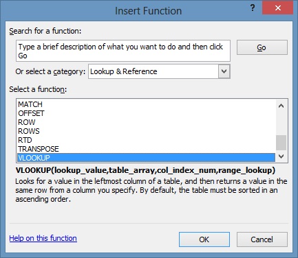
- To begin operation of the function, click the function button
 located above the cell field and adjacent to the formula bar.
 - In the "select a category" subfield, select Lookup & Reference.
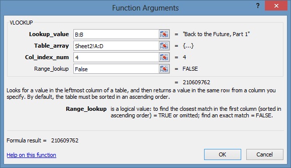
- In the now open "Function Arguments" window, click inside the Lookup_value field. This field requires a common element among both tabs as a reference, such as names, titles, years, etc. Click on the column letter on the primary sheet to select the entire column of the reference variable.
- Click into the Table_array field. The Table_array field requires information from the sheet containing the supplemental information. Click onto the sheet with the additional data. Highlight the columns from column A to the column of the desired data.
- Click into the Col_index_num field. Enter the total amount of columns selected for Table_array.
- Click into the Range_lookup field. Enter "False" into the field to allow the result to be an exact data match.
- Click "Ok" to activate the function. If entered correctly, the result will feature the data from sheet 2 associated with the reference variable.
Did You Know?
If you want to keep the results of the VLOOKUP and delete sheet 2, simply copy all the VLOOKUP results then right-click and select Paste Special. Select "Values" and click "Ok." Now you can delete sheet 2 without losing the results of the function.